3 Square Root
3.1 Square Root
As we saw in Chapter 2 about logarithms, we sometimes have to deal with highly skewed data. Square roots are another way to deal with this issue, with some different pros and cons that make it better to use us in some situations. We will spend our time in this section to talk about what those are.
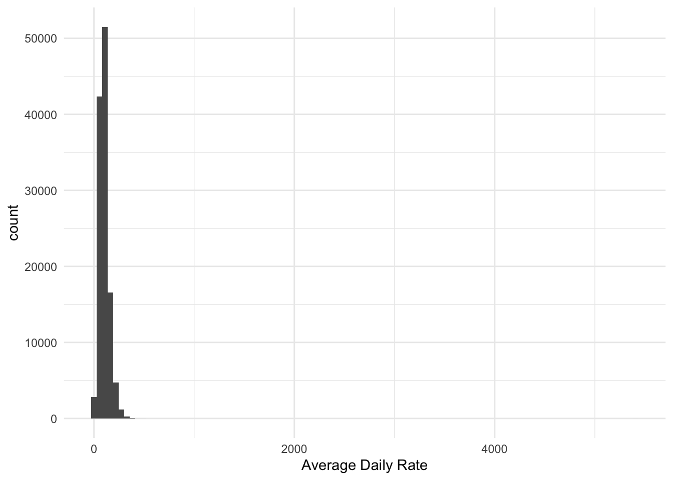
Below is a histogram of the average daily rate of the number of hotel stays. It is clear to see that this is another case where the data is highly skewed, with many values close to zero, but a few in the thousands.
This variable contains some negative values with the smallest being -6.38. We wouldn’t want to throw out the negative values. And we could think of many situations where both negative and positive values are part of a skewed distribution, especially financial. Bank account balances, delivery times, etc etc.
We need a method that transforms the scale to un-skew and also works with negative data. The square root could be what we are looking for. By itself, it takes as its input a positive number and returns the number that when multiplied by itself equals the input. This has the desired shrinking effect, where larger values are shrunk more than smaller values. Additionally, since its domain is the positive numbers (0 is a special case since it maps to itself) we can mirror it to work on negative numbers in the same way it worked on positive numbers. This gives us the signed square root
\[ y = \text{sign}(x)\sqrt{\left| x \right|} \]
Below we see the results of applying the signed square root.
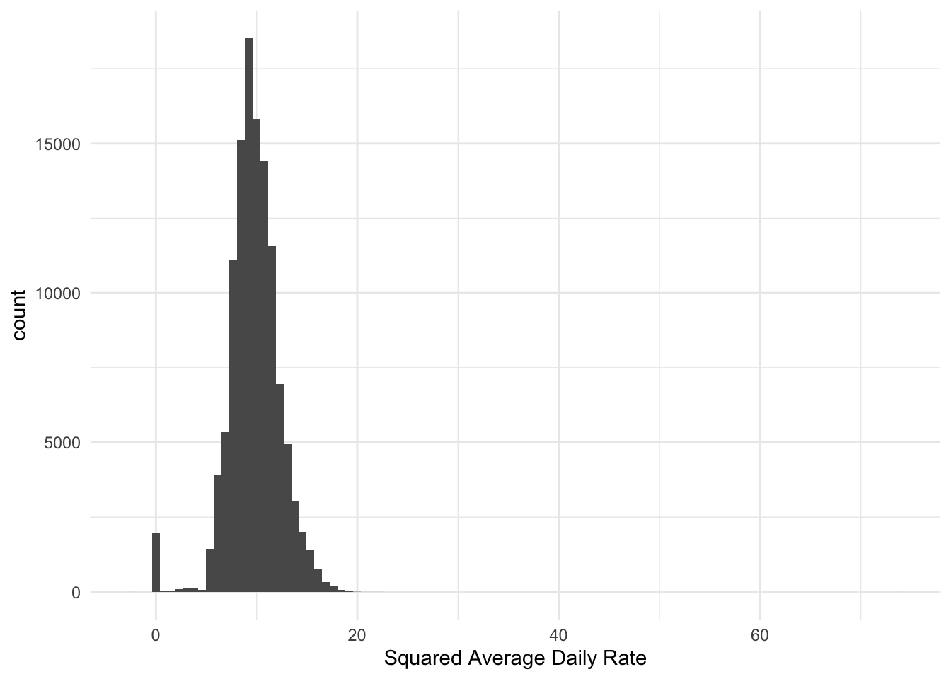
it is important to note that we are not trying to make the variable normally distributed. What we are trying to accomplish is to remove the skewed nature of the variable. Likewise, this method should not be used as a variance reduction tool as that task is handled by doing normalization which we start exploring more in Section 1.3.
It doesn’t have the same power to shrink large values as logarithms do, but it will seamlessly work with negative values and it would allow you to pick up on quadratic effects that you wouldn’t otherwise be able to pick up if you hadn’t applied the transformation. It also doesn’t have good inferential properties. It preserves the order of the numeric values, but it doesn’t give us a good way to interpret changes.
3.2 Pros and Cons
3.2.1 Pros
- A non-trained operation, can easily be applied to training and testing data sets alike
- Can be applied to all numbers, not just non-negative values
3.2.2 Cons
- It will leave regression coefficients virtually uninterpretable
- Is not a universal fix. While it can make skewed distributions less skewed. It has the opposite effect on a distribution that isn’t skewed
3.3 R Examples
We will be using the hotel_bookings data set for these examples.
library(recipes)

hotel_bookings |>
  select(lead_time, adr)
# A tibble: 119,390 × 2
lead_time adr
<dbl> <dbl>
1 342 0
2 737 0
3 7 75
4 13 75
5 14 98
6 14 98
7 0 107
8 9 103
9 85 82
10 75 106.
# ℹ 119,380 more rows{recipes} provides a step to perform logarithms, which out of the box uses \(e\) as the base with an offset of 0.
sqrt_rec <- recipe(lead_time ~ adr, data = hotel_bookings) |>
  step_sqrt(adr)

sqrt_rec |>
  prep() |>
  bake(new_data = NULL)
Warning in sqrt(new_data[[col_name]]): NaNs produced# A tibble: 119,390 × 2
adr lead_time
<dbl> <dbl>
1 0 342
2 0 737
3 8.66 7
4 8.66 13
5 9.90 14
6 9.90 14
7 10.3 0
8 10.1 9
9 9.06 85
10 10.3 75
# ℹ 119,380 more rowsif you want to do a signed square root instead, you can use step_mutate() which allows you to do any kind of transformations
signed_sqrt_rec <- recipe(lead_time ~ adr, data = hotel_bookings) |>
  step_mutate(adr = sqrt(abs(adr)) * sign(adr))

signed_sqrt_rec |>
  prep() |>
  bake(new_data = NULL)
# A tibble: 119,390 × 2
adr lead_time
<dbl> <dbl>
1 0 342
2 0 737
3 8.66 7
4 8.66 13
5 9.90 14
6 9.90 14
7 10.3 0
8 10.1 9
9 9.06 85
10 10.3 75
# ℹ 119,380 more rows3.4 Python Examples
We are using the ames data set for examples. Since there isn’t a built-in transformer for square root, we can create our own using FunctionTransformer() and numpy.sqrt().
from feazdata import ames
from sklearn.compose import ColumnTransformer
from sklearn.preprocessing import FunctionTransformer
import numpy as np

sqrt_transformer = FunctionTransformer(np.sqrt)

ct = ColumnTransformer(
    [('sqrt', sqrt_transformer, ['Wood_Deck_SF'])],
    remainder="passthrough")

ct.fit(ames)
ColumnTransformer(remainder='passthrough',
transformers=[('sqrt',
FunctionTransformer(func=<ufunc 'sqrt'>),
['Wood_Deck_SF'])])In a Jupyter environment, please rerun this cell to show the HTML representation or trust the notebook. On GitHub, the HTML representation is unable to render, please try loading this page with nbviewer.org.
ColumnTransformer(remainder='passthrough',
                  transformers=[('sqrt',
                                 FunctionTransformer(func=<ufunc 'sqrt'>),
['Wood_Deck_SF'])])['Wood_Deck_SF']
FunctionTransformer(func=<ufunc 'sqrt'>)
['MS_SubClass', 'MS_Zoning', 'Lot_Frontage', 'Lot_Area', 'Street', 'Alley', 'Lot_Shape', 'Land_Contour', 'Utilities', 'Lot_Config', 'Land_Slope', 'Neighborhood', 'Condition_1', 'Condition_2', 'Bldg_Type', 'House_Style', 'Overall_Cond', 'Year_Built', 'Year_Remod_Add', 'Roof_Style', 'Roof_Matl', 'Exterior_1st', 'Exterior_2nd', 'Mas_Vnr_Type', 'Mas_Vnr_Area', 'Exter_Cond', 'Foundation', 'Bsmt_Cond', 'Bsmt_Exposure', 'BsmtFin_Type_1', 'BsmtFin_SF_1', 'BsmtFin_Type_2', 'BsmtFin_SF_2', 'Bsmt_Unf_SF', 'Total_Bsmt_SF', 'Heating', 'Heating_QC', 'Central_Air', 'Electrical', 'First_Flr_SF', 'Second_Flr_SF', 'Gr_Liv_Area', 'Bsmt_Full_Bath', 'Bsmt_Half_Bath', 'Full_Bath', 'Half_Bath', 'Bedroom_AbvGr', 'Kitchen_AbvGr', 'TotRms_AbvGrd', 'Functional', 'Fireplaces', 'Garage_Type', 'Garage_Finish', 'Garage_Cars', 'Garage_Area', 'Garage_Cond', 'Paved_Drive', 'Open_Porch_SF', 'Enclosed_Porch', 'Three_season_porch', 'Screen_Porch', 'Pool_Area', 'Pool_QC', 'Fence', 'Misc_Feature', 'Misc_Val', 'Mo_Sold', 'Year_Sold', 'Sale_Type', 'Sale_Condition', 'Sale_Price', 'Longitude', 'Latitude']
passthrough
ct.transform(ames) sqrt__Wood_Deck_SF ... remainder__Latitude
0 14.491 ... 42.054
1 11.832 ... 42.053
2 19.824 ... 42.053
3 0.000 ... 42.051
4 14.560 ... 42.061
... ... ... ...
2925 10.954 ... 41.989
2926 12.806 ... 41.988
2927 8.944 ... 41.987
2928 15.492 ... 41.991
2929 13.784 ... 41.989
[2930 rows x 74 columns]We can also create and perform a signed square root transformation, by creating a function for signed_sqrt() and then using it in FunctionTransformer() as before
def signed_sqrt(x):
  return np.sqrt(np.abs(x)) * np.sign(x)

signed_sqrt_transformer = FunctionTransformer(signed_sqrt)

ct = ColumnTransformer(
    [('signed_sqrt', signed_sqrt_transformer, ['Wood_Deck_SF'])],
    remainder="passthrough")

ct.fit(ames)
ColumnTransformer(remainder='passthrough',
transformers=[('signed_sqrt',
FunctionTransformer(func=<function signed_sqrt at 0x2ad805a80>),
['Wood_Deck_SF'])])In a Jupyter environment, please rerun this cell to show the HTML representation or trust the notebook. On GitHub, the HTML representation is unable to render, please try loading this page with nbviewer.org.
ColumnTransformer(remainder='passthrough',
                  transformers=[('signed_sqrt',
                                 FunctionTransformer(func=<function signed_sqrt at 0x2ad805a80>),
['Wood_Deck_SF'])])['Wood_Deck_SF']
FunctionTransformer(func=<function signed_sqrt at 0x2ad805a80>)
['MS_SubClass', 'MS_Zoning', 'Lot_Frontage', 'Lot_Area', 'Street', 'Alley', 'Lot_Shape', 'Land_Contour', 'Utilities', 'Lot_Config', 'Land_Slope', 'Neighborhood', 'Condition_1', 'Condition_2', 'Bldg_Type', 'House_Style', 'Overall_Cond', 'Year_Built', 'Year_Remod_Add', 'Roof_Style', 'Roof_Matl', 'Exterior_1st', 'Exterior_2nd', 'Mas_Vnr_Type', 'Mas_Vnr_Area', 'Exter_Cond', 'Foundation', 'Bsmt_Cond', 'Bsmt_Exposure', 'BsmtFin_Type_1', 'BsmtFin_SF_1', 'BsmtFin_Type_2', 'BsmtFin_SF_2', 'Bsmt_Unf_SF', 'Total_Bsmt_SF', 'Heating', 'Heating_QC', 'Central_Air', 'Electrical', 'First_Flr_SF', 'Second_Flr_SF', 'Gr_Liv_Area', 'Bsmt_Full_Bath', 'Bsmt_Half_Bath', 'Full_Bath', 'Half_Bath', 'Bedroom_AbvGr', 'Kitchen_AbvGr', 'TotRms_AbvGrd', 'Functional', 'Fireplaces', 'Garage_Type', 'Garage_Finish', 'Garage_Cars', 'Garage_Area', 'Garage_Cond', 'Paved_Drive', 'Open_Porch_SF', 'Enclosed_Porch', 'Three_season_porch', 'Screen_Porch', 'Pool_Area', 'Pool_QC', 'Fence', 'Misc_Feature', 'Misc_Val', 'Mo_Sold', 'Year_Sold', 'Sale_Type', 'Sale_Condition', 'Sale_Price', 'Longitude', 'Latitude']
passthrough
ct.transform(ames) signed_sqrt__Wood_Deck_SF ... remainder__Latitude
0 14.491 ... 42.054
1 11.832 ... 42.053
2 19.824 ... 42.053
3 0.000 ... 42.051
4 14.560 ... 42.061
... ... ... ...
2925 10.954 ... 41.989
2926 12.806 ... 41.988
2927 8.944 ... 41.987
2928 15.492 ... 41.991
2929 13.784 ... 41.989
[2930 rows x 74 columns]